← All research projects

Published · ApJ, 2026

Particle acceleration in magnetized shear-driven turbulence

How a turbulent shear layer turns a sequence of small, random kicks into a high-energy particle population.

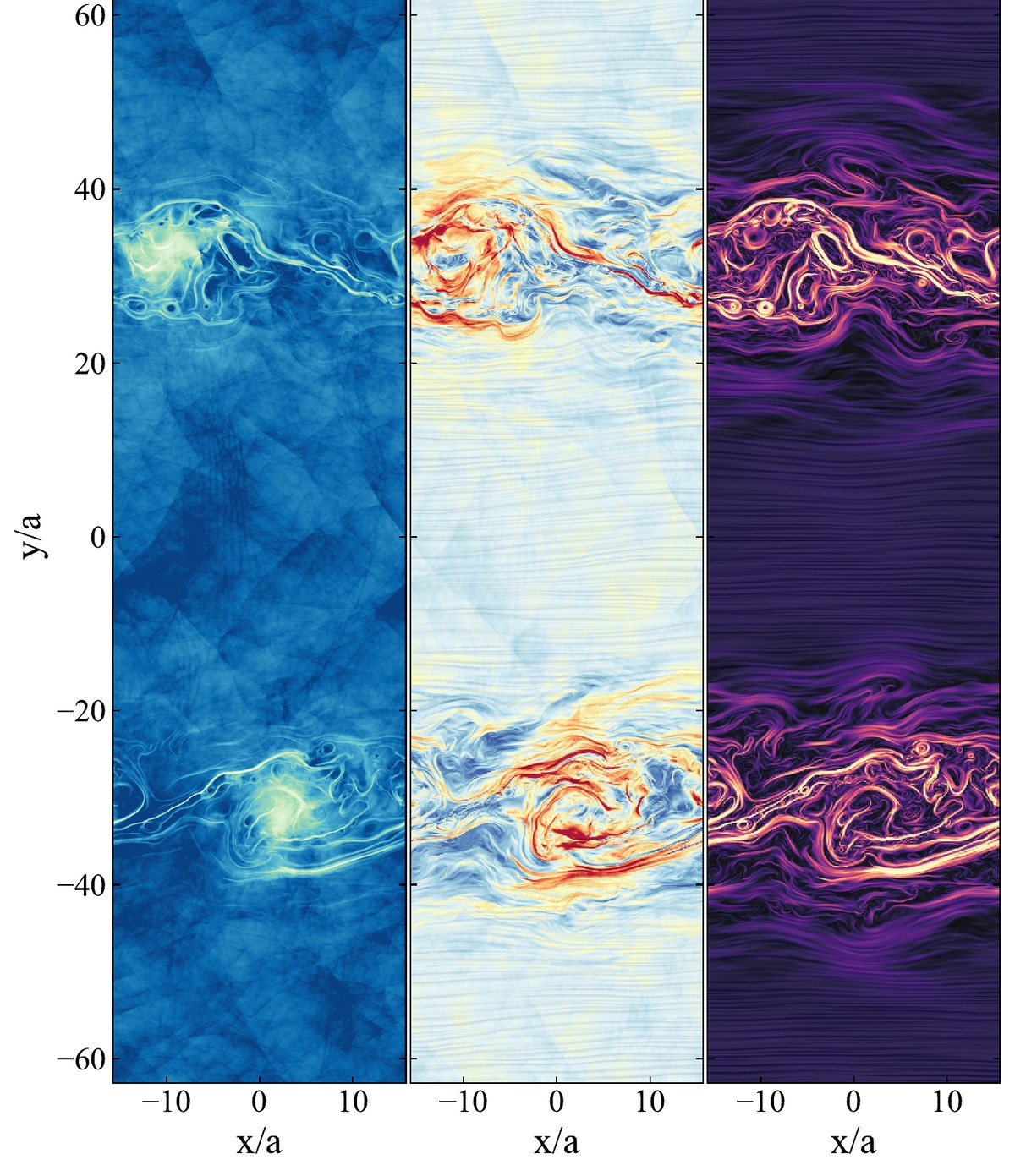
Three side-by-side simulation maps of a shear layer in its turbulent steady state,
                      showing gas density, velocity magnitude and magnetic field strength.
A shear-driven turbulent layer in its statistically steady state: density (left), velocity (middle) and magnetic field strength (right). The field is stretched and folded into thin, bright filaments wherever the flow is most strongly sheared.

Wherever one parcel of plasma slides past another, the interface between them is unstable. The Kelvin–Helmholtz instability curls it into vortices, those break down into turbulence, and the turbulence drags the magnetic field into a tangle. This happens at the edge of a jet, along gas stripped from an infalling galaxy, at the boundary of a wind. What I wanted to know is what the tangle does to the charged particles threading through it.

We simulated particle acceleration in sustained, subsonic, non-relativistic magnetized turbulence driven purely by velocity shear, with the particles allowed to push back on the fluid. Whether the turbulence is being fed turns out to matter a great deal. Keep stirring and the particles go on gaining energy indefinitely. Stop, and the turbulence drains its own reservoirs within a few eddy turnover times, and acceleration stops with it.

The mechanism is really just geometry. A turbulent electric field distorts a particle’s gyro-orbit. On the half-cycle where the force accelerates it, the particle travels further along that force and gains more; on the half-cycle where the force decelerates it, the path is shorter and it loses less. Averaged over many random kicks the asymmetry leaves a net gain, and that gain scales with the square of the shear velocity, which is what second-order Fermi acceleration looks like.
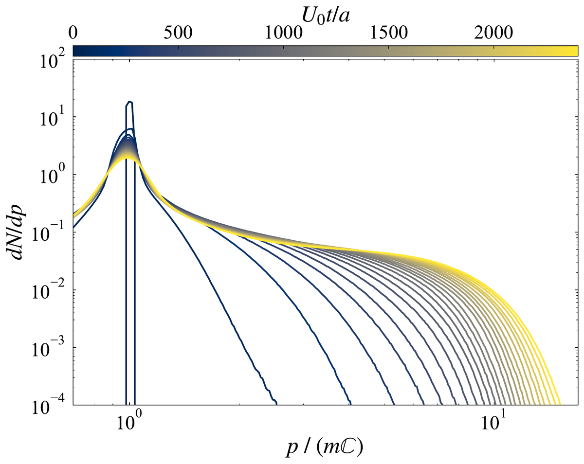
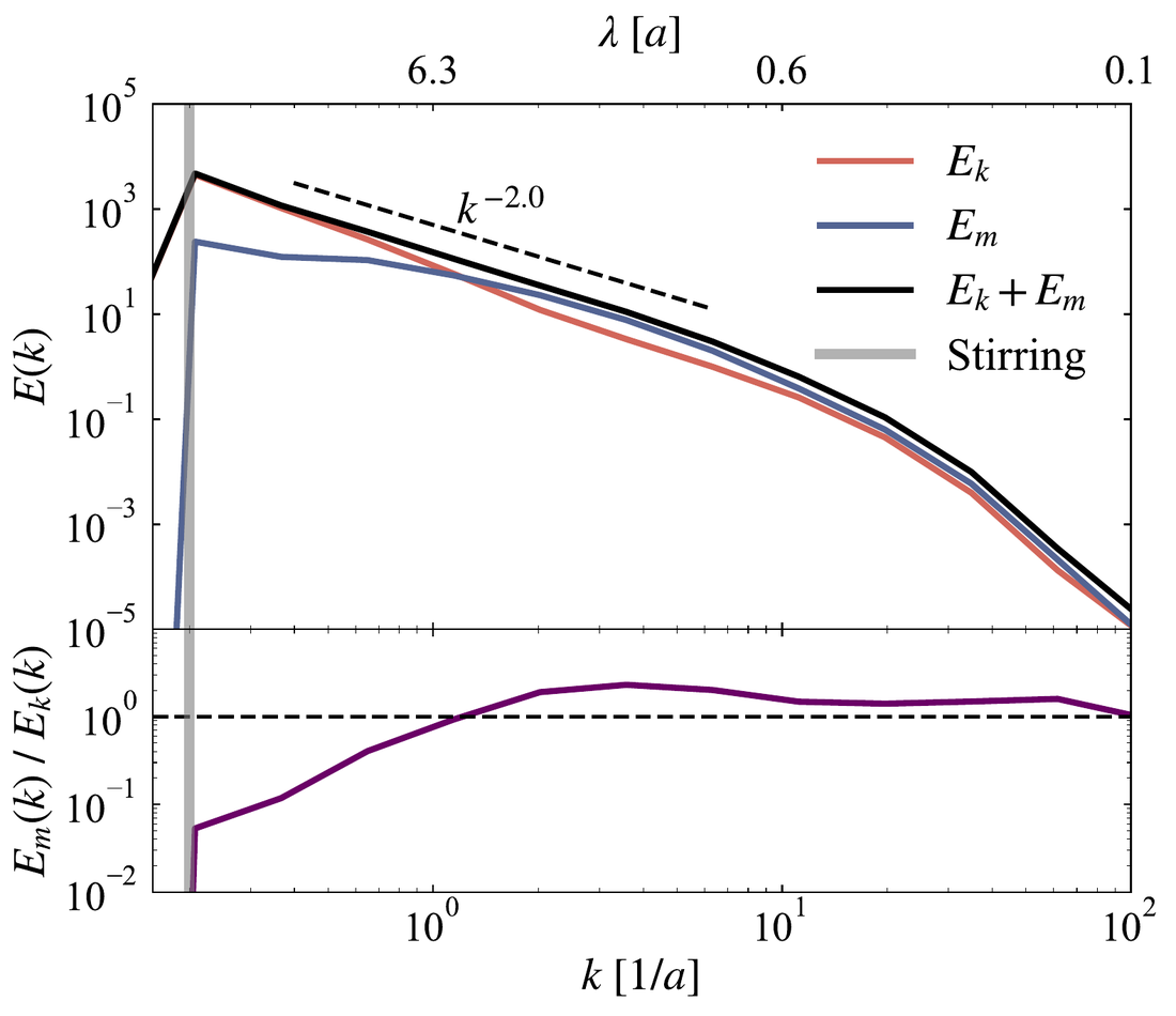
An initially monoenergetic population grows a substantial non-thermal tail. Particles that repeatedly cross the shear layers gain energy by what is essentially geometric Brownian motion, which gives a log-normal momentum distribution. Once their gyroradii outgrow the turbulent layer they turn preferentially perpendicular to the background field.

Published in The Astrophysical Journal 1009, 247 (2026).
2D MHD particle-in-cell simulations using the MHD-PIC module (Sun & Bai 2023) of Athena++.

Particle momentum distribution at successive times, showing an initially sharp
                    peak developing an extended high-energy tail.
The particle momentum distribution, color-coded by time. The initially monoenergetic spike flattens into a broad non-thermal tail whose high-energy cutoff keeps advancing for as long as the turbulence is driven.
Kinetic and magnetic energy power spectra of the turbulence versus wavenumber,
                    with a k to the minus two reference slope.
Kinetic and magnetic energy spectra of the steady-state turbulence. The inertial range follows a k−2 slope, and magnetic energy overtakes kinetic energy at small scales.
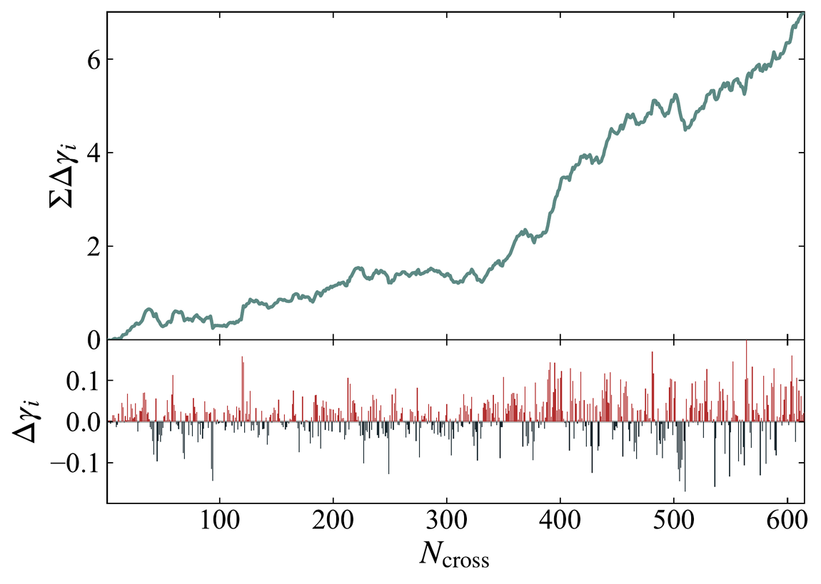
Top: the running sum of a particle's energy changes over 600 shear-layer crossings,
                    climbing unevenly from 0 to about 7. Bottom: the individual per-crossing changes,
                    with gains in red and losses in black, of comparable size.
One particle's energy, crossing by crossing. The bottom panel is the gain or loss at each crossing of a shear layer, and the red gains and black losses look almost symmetric. The top panel is their running total. The gains are very slightly larger on average, and 600 crossings later that small bias has compounded into a factor of several in energy.
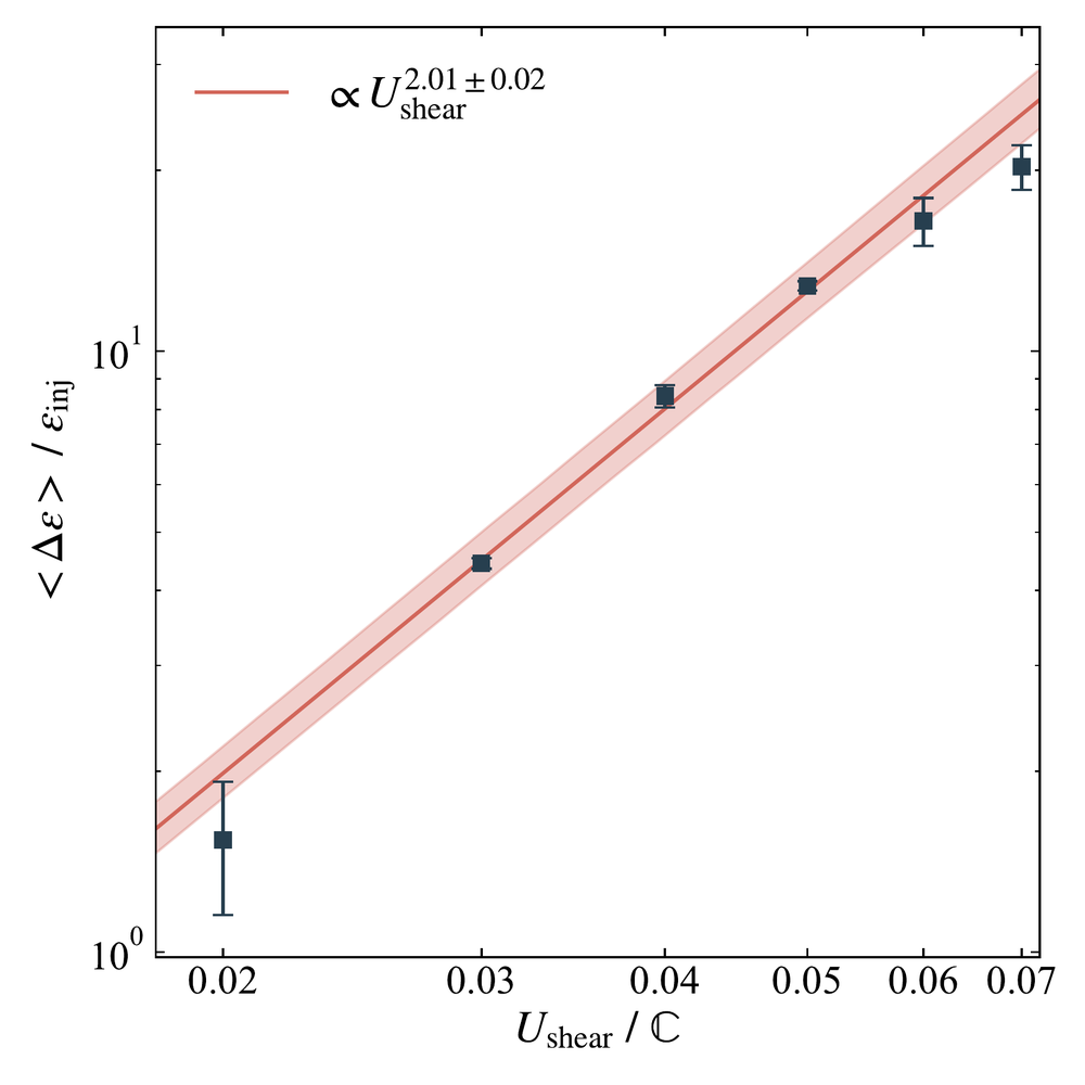
Mean fractional energy gain per particle plotted against shear velocity on log axes,
                    with a fitted power law of slope 2.01 plus or minus 0.02.
Repeating that measurement across shear velocities. The mean energy gain scales as the shear velocity to the power 2.01 ± 0.02. A power of two is what second-order Fermi acceleration predicts, which is how we know that is the mechanism at work.
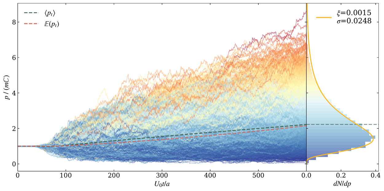
Hundreds of particle momentum trajectories fanning out from a common starting value,
                  colored blue to red by final momentum, with the resulting log-normal distribution
                  plotted at the right.
The same process for every particle that crosses the layers repeatedly. All of them start at the same momentum and fan out into the spread on the right, which is log-normal, the distribution you get from multiplying many small random factors together. The dashed lines are the measured and predicted means.