Research

I run simulations of turbulent, magnetized plasmas: how the turbulence is driven, where its energy ends up, and what it does to the cosmic rays and the cold gas embedded in it. Two of these projects are published, two are underway.

Starting now

Cosmic-ray transport and feedback

Cosmic rays carry a large share of the energy that supernovae and AGN put back into a galaxy. They cool slowly and stay tied to magnetized gas, so they can move energy far from where they were accelerated, drive winds, and suppress star formation. How much they actually do depends on one microphysical number: how often they scatter off magnetic fluctuations. That number sets how fast they travel relative to the gas and how hard they push on it.

At the moment galaxy-scale models put that number in by hand. I want to compute it instead, at the two ends of the range that bracket the bulk of the Galactic cosmic-ray population: close to a source, where the cosmic rays are dense enough to amplify their own scattering field, and far from one, in cold partially ionized gas, where collisions between ions and neutrals damp the waves that would normally do the scattering and whatever deflection survives has to come from the geometry of the field itself.

Both cases use the same tool and the same diagnostic: MHD particle-in-cell simulations in Athena++, with the parallel diffusion coefficient measured directly from the particles, so the two regimes are measured on the same footing.
In progress

Turbulence in multiphase gas

Hot and cold gas coexist almost everywhere it matters: in cluster cores, in the circumgalactic medium, in the interstellar medium. The cold phase is much denser, much colder, and radiates away far more energy than you would naively expect it to receive, which means something has to keep supplying it. Turbulence is the obvious candidate, but the path from large-scale stirring to heat in a thin cold filament runs through physics that ideal simulations cannot resolve.

I am running simulations of driven turbulence in a radiatively cooling, thermally unstable plasma to follow that path with the dissipation treated explicitly rather than left to the grid. The work is still in progress, so I will leave the details until there is a paper to point at.

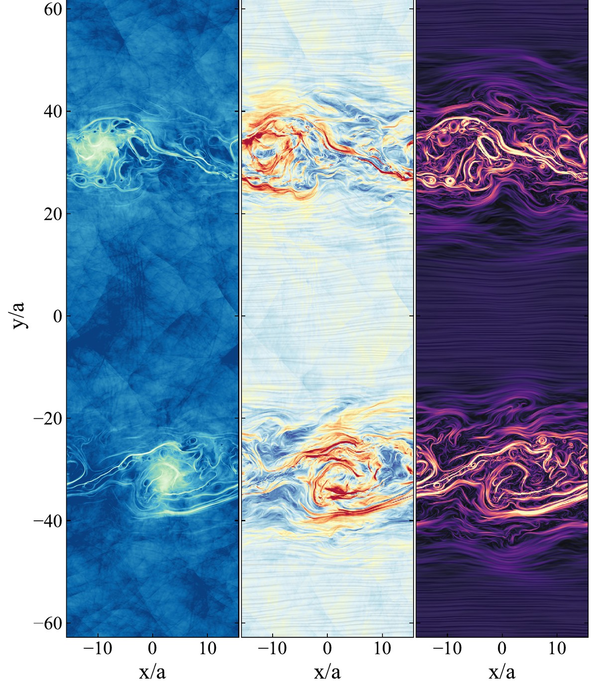
Three side-by-side simulation maps of a shear layer in its turbulent steady state,
                      showing gas density, velocity magnitude and magnetic field strength.
A shear-driven turbulent layer in its statistically steady state: density (left), velocity (middle) and magnetic field strength (right). The field is stretched and folded into thin, bright filaments wherever the flow is most strongly sheared.

Published work

Particle acceleration in magnetized shear-driven turbulence

Wherever one parcel of plasma slides past another, the interface between them is unstable. The Kelvin–Helmholtz instability curls it into vortices, those break down into turbulence, and the turbulence drags the magnetic field into a tangle. This happens at the edge of a jet, along gas stripped from an infalling galaxy, at the boundary of a wind. What I wanted to know is what the tangle does to the charged particles threading through it.

We simulated particle acceleration in sustained, subsonic, non-relativistic magnetized turbulence driven purely by velocity shear, with the particles allowed to push back on the fluid. Whether the turbulence is being fed turns out to matter a great deal. Keep stirring and the particles go on gaining energy indefinitely. Stop, and the turbulence drains its own reservoirs within a few eddy turnover times, and acceleration stops with it.

The mechanism is really just geometry. A turbulent electric field distorts a particle’s gyro-orbit. On the half-cycle where the force accelerates it, the particle travels further along that force and gains more; on the half-cycle where the force decelerates it, the path is shorter and it loses less. Averaged over many random kicks the asymmetry leaves a net gain, and that gain scales with the square of the shear velocity, which is what second-order Fermi acceleration looks like.

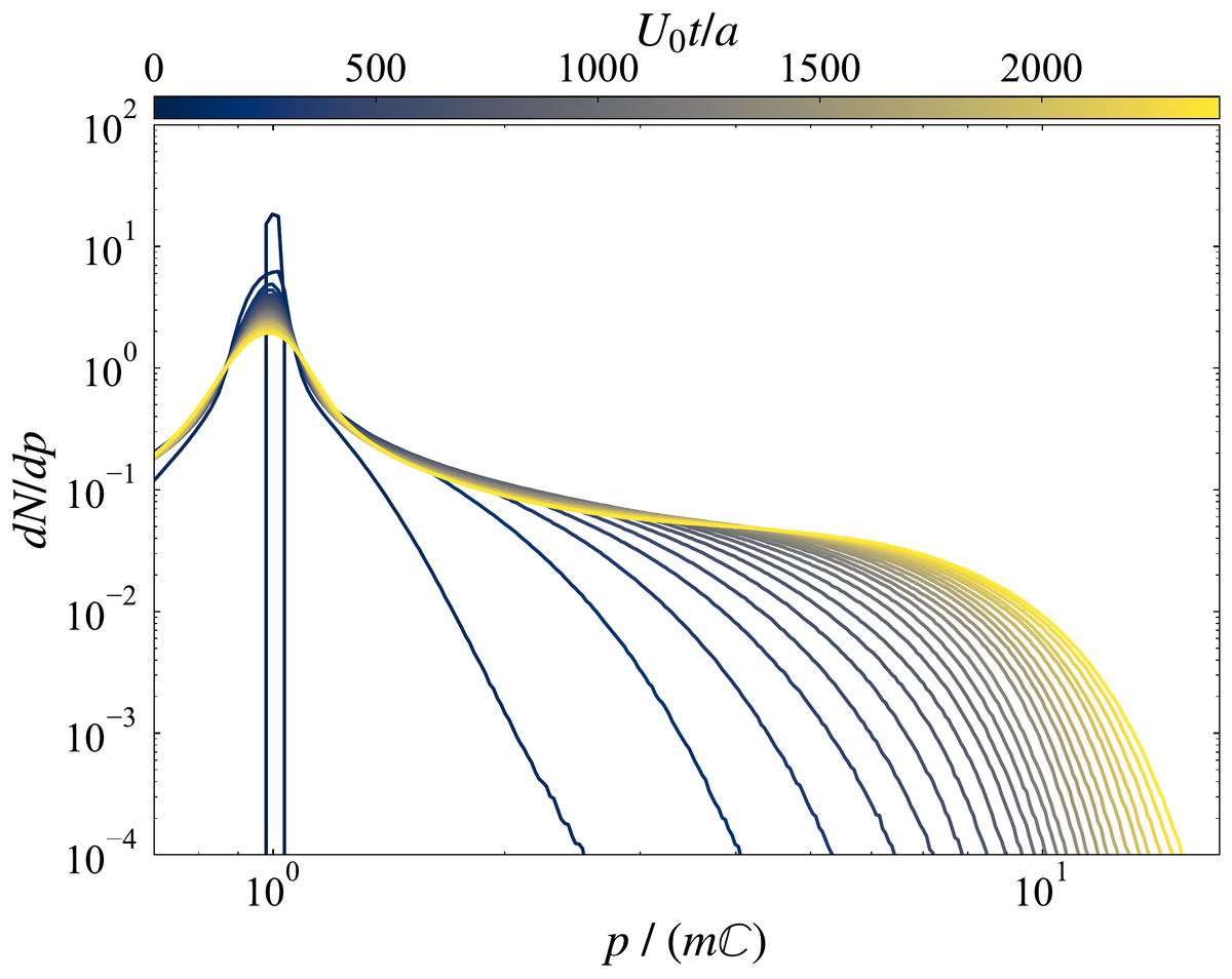
An initially monoenergetic population grows a substantial non-thermal tail. Particles that repeatedly cross the shear layers gain energy by what is essentially geometric Brownian motion, which gives a log-normal momentum distribution. Once their gyroradii outgrow the turbulent layer they turn preferentially perpendicular to the background field.

2D MHD particle-in-cell simulations using the MHD-PIC module (Sun & Bai 2023) of Athena++.

Particle momentum distribution at successive times, showing an initially sharp
                    peak developing an extended high-energy tail.
The particle momentum distribution, color-coded by time. The initially monoenergetic spike flattens into a broad non-thermal tail whose high-energy cutoff keeps advancing for as long as the turbulence is driven.
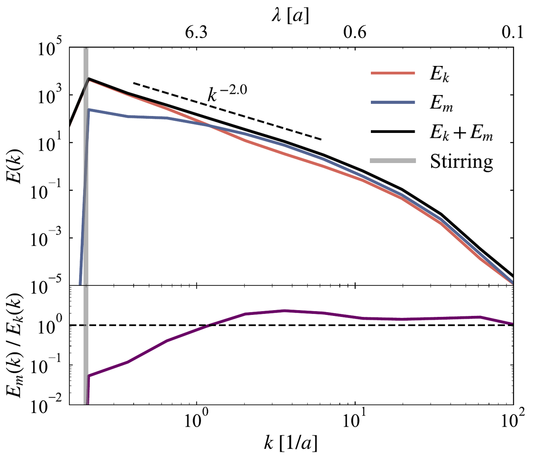
Kinetic and magnetic energy power spectra of the turbulence versus wavenumber,
                    with a k to the minus two reference slope.
Kinetic and magnetic energy spectra of the steady-state turbulence. The inertial range follows a k−2 slope, and magnetic energy overtakes kinetic energy at small scales.
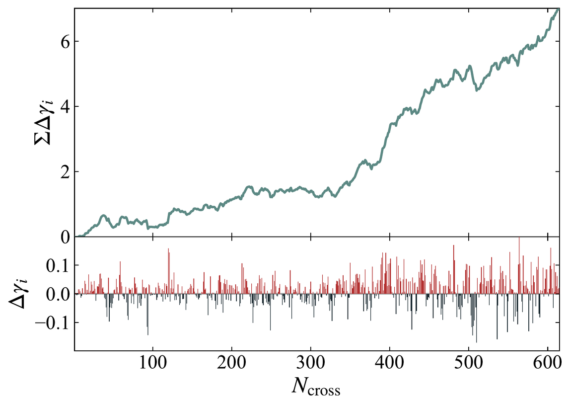
Top: the running sum of a particle's energy changes over 600 shear-layer crossings,
                    climbing unevenly from 0 to about 7. Bottom: the individual per-crossing changes,
                    with gains in red and losses in black, of comparable size.
One particle's energy, crossing by crossing. The bottom panel is the gain or loss at each crossing of a shear layer, and the red gains and black losses look almost symmetric. The top panel is their running total. The gains are very slightly larger on average, and 600 crossings later that small bias has compounded into a factor of several in energy.
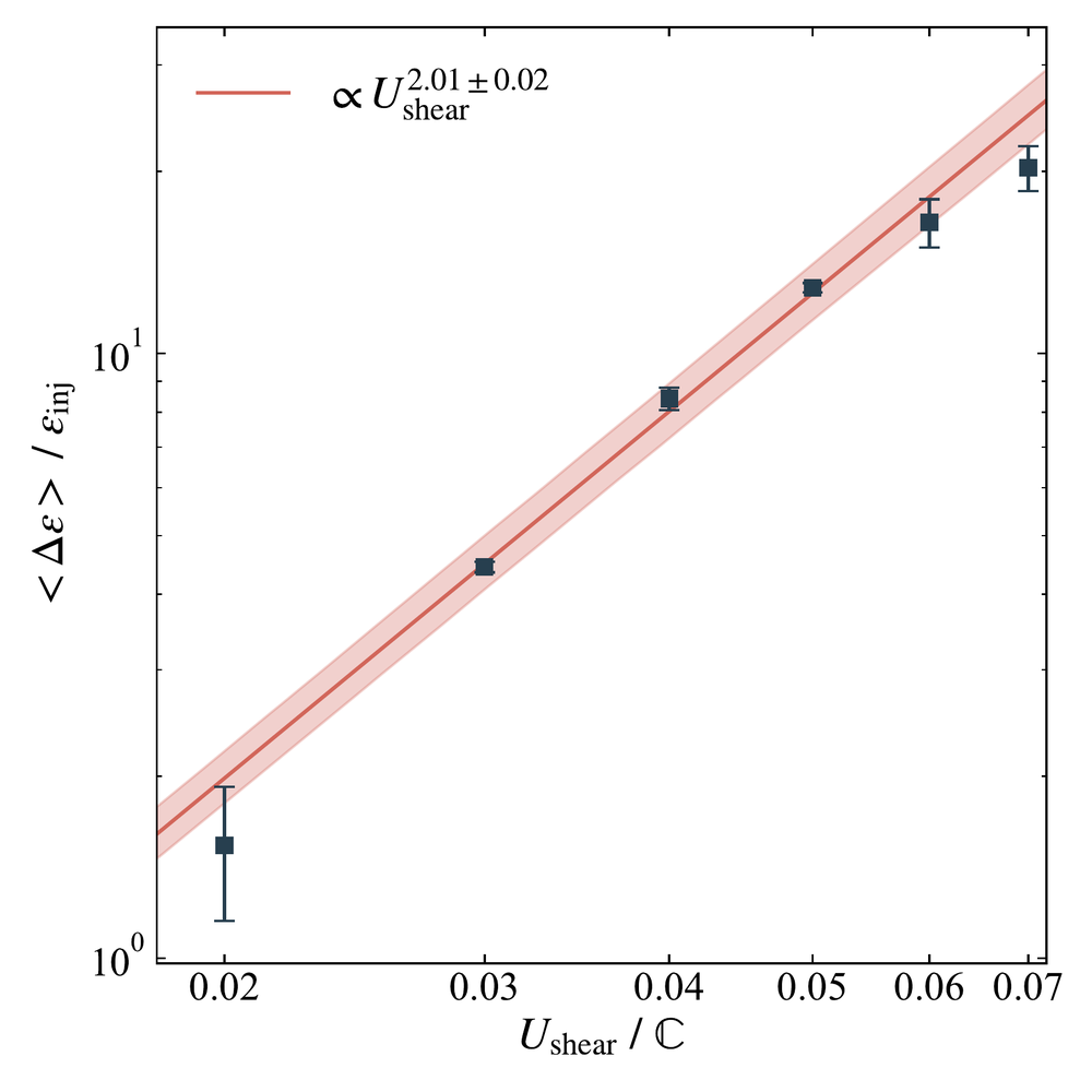
Mean fractional energy gain per particle plotted against shear velocity on log axes,
                    with a fitted power law of slope 2.01 plus or minus 0.02.
Repeating that measurement across shear velocities. The mean energy gain scales as the shear velocity to the power 2.01 ± 0.02. A power of two is what second-order Fermi acceleration predicts, which is how we know that is the mechanism at work.
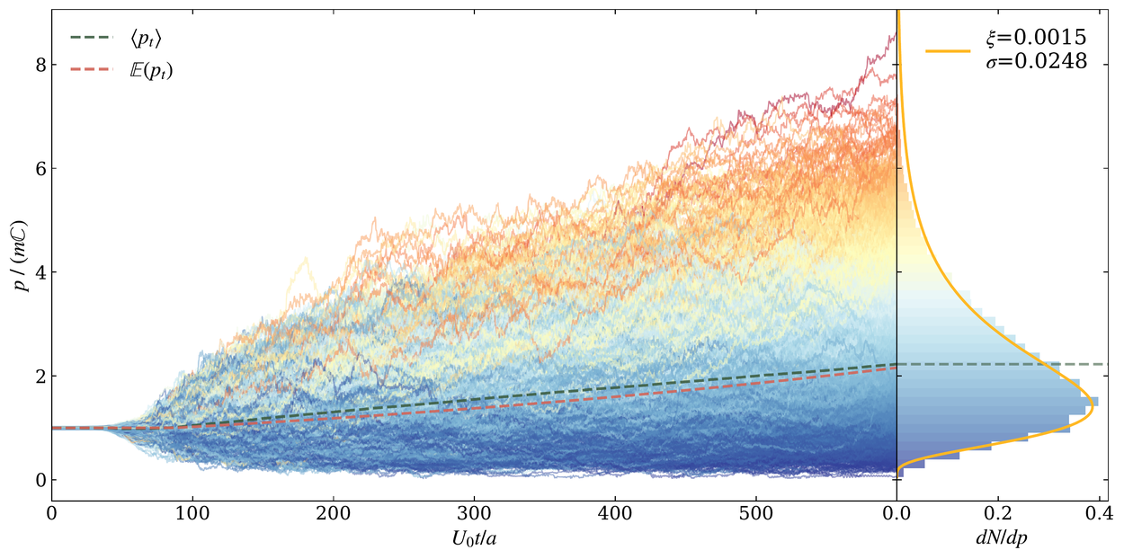
Hundreds of particle momentum trajectories fanning out from a common starting value,
                  colored blue to red by final momentum, with the resulting log-normal distribution
                  plotted at the right.
The same process for every particle that crosses the layers repeatedly. All of them start at the same momentum and fan out into the spread on the right, which is log-normal, the distribution you get from multiplying many small random factors together. The dashed lines are the measured and predicted means.
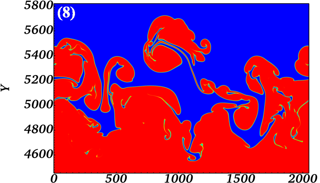
Simulation snapshot of a Rayleigh-Taylor unstable flame front, with burnt fluid
                      in red rising into unburnt fluid in blue as large mushroom-shaped bubbles.
A Rayleigh–Taylor unstable flame deep in the chaotic burning regime. Burnt fluid (red) rises into unburnt fluid (blue) as bubbles that merge and grow without bound.

Undergraduate work

Rayleigh–Taylor unstable flames and the inverse cascade

Put a light fluid underneath a heavy one and the interface between them goes unstable: bubbles rise, spikes fall, and small wrinkles merge into larger ones. That merging, an inverse cascade in wavenumber, is what makes the classical Rayleigh–Taylor mixing layer forget its initial conditions and settle into self-similar growth. We wanted to know whether a burning interface forgets in the same way.

It does not, or at least not straightforwardly. A reacting front can stabilize itself: perturb a model flame with a single mode and it stops growing, locking into a steady traveling wave that can persist almost indefinitely. We perturbed it with two instead, a large-amplitude primary mode k1 and a smaller secondary mode k2, and looked at what it takes to break that stalemate.

Early on the two modes ignore each other and the flame propagates as a metastable traveling wave. Once the secondary mode has grown large enough they couple, the traveling wave is destabilized, and the bubbles take off. What the coupling produces is a long-wavelength mode whose wavenumber is the greatest common divisor of the two you started with.

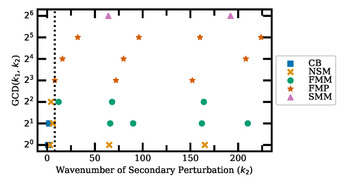
We found five distinct flame-growth solution types, selected by GCD(k1k2). Depending on that one number the flame may stall, develop coherent pulsations, settle back into a metastable traveling wave, or run away into chaotic burning. The same two-mode dynamics show up in ablative and classical Rayleigh–Taylor, which suggests all three share a mode-coupling mechanism.

Direct numerical simulations of a 2D Boussinesq premixed model flame with Nek5000, a spectral-element CFD code: 512 × 2304 elements at spectral order N = 9.

Phase diagram of flame solution types plotted against secondary-mode wavenumber
                    and the greatest common divisor of the two wavenumbers.
The solution-type phase diagram. Which of the five behaviors a flame picks depends on GCD(k1k2), not on k2 itself.
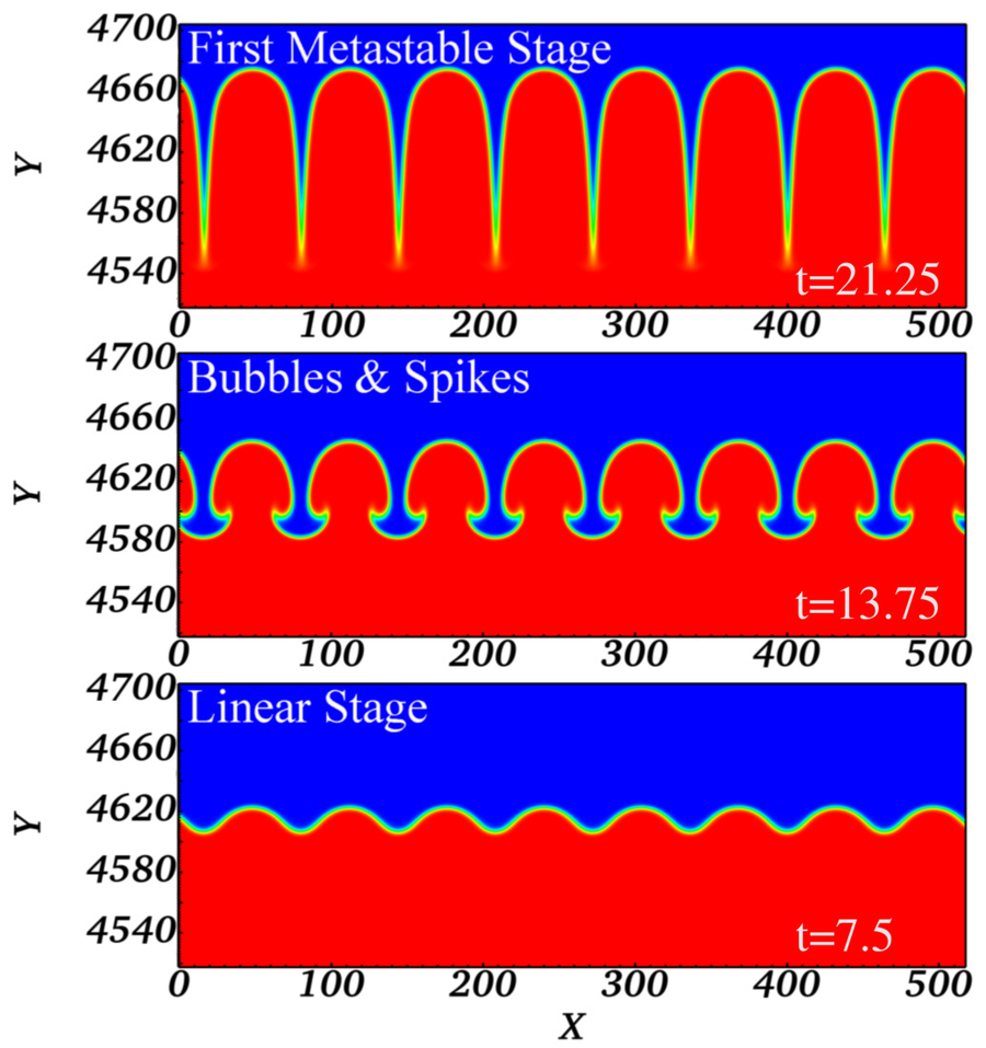
Three stacked snapshots showing a flame front growing from a small sinusoidal
                    perturbation into bubbles and spikes, then stabilising.
The early stage: a small perturbation grows exponentially, bubbles and spikes form, and the flame settles into the metastable traveling wave that two-mode coupling later breaks.

Codes and computing

The plasma work uses the MHD particle-in-cell module of Athena++, which evolves the background fluid with MHD while treating the energetic particles kinetically. The flames work used Nek5000, a spectral-element code, at 512 × 2304 elements and order N = 9. Both ran on NSF-supported machines through XSEDE and ACCESS, and the analysis is Python.

Setups, the analysis package and the figure scripts for the flames paper are on Zenodo under GPL-3.0: 10.5281/zenodo.13750992.